PINN PDE Solver
Physics-informed neural network solving the heat equation to 2.5×10⁻⁴ error, with an MLOps gate.
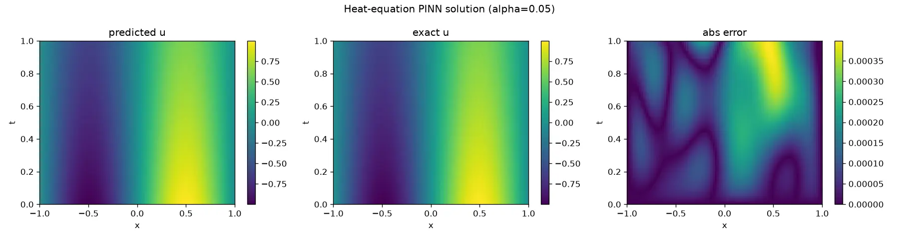
A PDE solver is only half the work. Getting a trained model into production means proving it earned its place, and most research code has no gate that can say no.
A parametric PINN in JAX and Equinox trains on the PDE residual itself, with the initial and boundary conditions made exact by construction through a hard-constraint ansatz rather than soft loss penalties. Training runs as an Azure ML job, MLflow tracks parameters and metrics, and an evaluation gate decides promotion to the model registry.
2.5×10⁻⁴ mean relative L2 error against the analytical solution, across a continuous range of diffusivities. A deliberately under-trained model was run through the same gate and correctly rejected - nothing was registered.
A physics-informed neural network that solves the 1D heat equation to 2.48 × 10⁻⁴ mean relative L2 — measured on four interior diffusivities on a 100 x 100 grid against the closed-form solution — wrapped in an Azure ML pipeline whose decision point is an evaluation gate, so the model registry only ever contains models that earned their place.
What is it?
- A real solver. A parametric PINN in JAX/Equinox solves the 1D heat equation across a continuous
range of diffusivities
α ∈ [0.01, 0.1]— one network, infinitely many PDE instances — validated against the analytical solution to 2.48 × 10⁻⁴ mean relative L2 on the gate's four interior α. Across a dense 19-point sweep of the whole range the mean is 2.97 × 10⁻⁴, worst 1.26 × 10⁻³ at α = 0.01, where the network is extrapolating toward the edge of its training band. - A real pipeline. Training runs as an Azure ML command job; MLflow captures params/metrics/artifacts; an evaluation gate decides promotion; passing models land in a versioned Model Registry; one is served as a live REST endpoint.
- Gates, not just training loops. A deliberately under-trained config is run through the same gate and correctly rejected – nothing is registered. The registry's value is what it refuses to admit.
- Local-first. The identical train → gate → register scripts run against a local MLflow store with zero Azure dependency, so the whole thing is validated before any cloud round-trip.
- Cost-disciplined. CPU, scale-to-zero compute; the online endpoint was deployed, proven with a live call, then torn down – no resources left billing.
1. The science – a parametric PINN for the heat equation
The 1D heat equation with homogeneous Dirichlet boundaries and a sinusoidal initial profile:
∂u/∂t = α ∂²u/∂x²,    x ∈ [-1, 1],  t ∈ [0, 1]
u(x, 0) = sin(π x),   u(±1, t) = 0
A physics-informed network is trained not on labelled data but on the PDE residual itself – it
minimises how badly its own derivatives (taken with jax.grad) violate the equation at randomly sampled
collocation points. The model is parametric in α: inputs are [x, t, α], output is u, so a single
network represents the entire family of solutions over the diffusivity range.
Two engineering decisions did the heavy lifting:
- Hard-constraint ansatz. Instead of penalising boundary/initial-condition violations softly in the
loss (where the optimiser trades them off against the residual), the output is structured as
u = sin(π x) + (1 − x²) · t · N(x, t, α). Att = 0this collapses tosin(π x); atx = ±1the(1 − x²)factor kills it. The IC and BCs are therefore exact by construction, and the networkNonly has to learn the interior dynamics. - Input normalisation.
αspans[0.01, 0.1], two orders of magnitude narrower thanxandt, so every input is normalised to ~[-1, 1]before the network sees it. Measured by ablation (identical seed, initialisation and collocation points, 2 000 epochs: 6.83 × 10⁻³ vs 1.45 × 10⁻² mean relative L2, so the raw-input model has about 2.1× the error, and is 1.3–3.7× worse at everyαtested. The ablation also ruled out the explanation this README used to give: the raw-input model does not collapse toward anα-averaged solution. It reproduces 96.4% of the trueα-sensitivity of the field, against 94.7% for the normalised model. Normalisation buys accuracy and faster early training (the raw arm's loss stalls near 2 × 10⁻² for its first ~500 epochs), not the ability to resolveα. This is a single seed at a reduced budget.
Breadth (in the core, outside the Azure ML pipeline): the same architecture also solves Burgers' equation
(nonlinear, validated against a method-of-lines numerical reference since it has no closed form) and an
inverse problem – recovering an unknown diffusivity α from sparse, noisy observations, a
parameter-estimation task a classical forward solver cannot do directly. Over 8 noise realisations the
recovered α has a spread of 4.25 × 10⁻⁴ against a Cramér–Rao floor of 2.44 × 10⁻⁴. With 8 noise
realisations the standard error on an estimated standard deviation is about 27%, so the ratio is
1.74 ± 0.47 — the estimator sits close to the information floor, but "close" is all this many seeds can
support.
How accuracy scales
How do you know the collocation budget is enough? A convergence study trains the network from a
fixed seed across a range of collocation-point counts – each through the same train() loop as
the headline model (cosine-annealed Adam) – and measures the mean relative L2 against the analytical
solution.
Reduced-budget study (2000 epochs per point; the headline model runs 20 000). Error falls from 1.368e-02 at 100 points to 9.285e-03 at 1000 points – roughly halving over that range – then plateaus: 2000 and 4000 points only reach 9.150e-03 and 8.982e-03, each under a 2% further drop versus 8–16% per doubling below 1000. Past that point the bottleneck is optimisation/network capacity, not collocation density. The slope, not the absolute level, is the finding: at the full 20 000-epoch budget the whole curve sits lower.
For Burgers', the "exact" field is itself a numerical (method-of-lines) reference, so it carries its own discretisation error. A grid-refinement check (nx = 512 vs nx = 2048, via puts that at rel-L2 4.32 × 10⁻³ — about 4.1% of the PINN's 0.105. The remaining error is the model's: a smooth tanh network smears the steep front at x = 0. Away from it (excluding |x| < 0.1) the PINN's relative L2 is 2.91 × 10⁻³, and its L∞ of 1.08 — on a field with |u| ≤ 1 — means it misses the jump essentially completely at the worst point. This is the textbook PINN failure mode on advection-dominated problems.
What was not tried here: L-BFGS polish after Adam, residual-adaptive collocation resampling near the front, causal or time-marching training, and a larger collocation budget (this run uses 2 000 points and Adam only). Raissi et al. report ~1e-3 on this benchmark with a soft-constraint formulation and L-BFGS. The Burgers model is included as breadth — a second, nonlinear PDE through the same architecture — not as a competitive result.